Topic Modelling With BERTopic

Topic modelling is a common task in NLP. It's an unsupervised technique for determining what topics, which can be thought of as categories, are part of a set of documents and what topics each document is likely to be a part of. Since it's an unsupervised technique, no labels are required, meaning we do not need a predefined list of topics – rather just the text from the documents. In this article, we'll discuss how to perform topic modelling with BERTopic, which is a leading Python package for this task and uses state-of-the-art Transformer models.

Topic modelling has a wide range of applications. For example, a social media site may want to know what news topics are currently trending but does not have a predefined list of the current news topics. By applying topic modelling, the site can determine what topics are trending along with what articles fall within them. This is just one of the countess examples of applying topic modelling, and in this tutorial we'll apply topic modelling to new headlines related to the economy

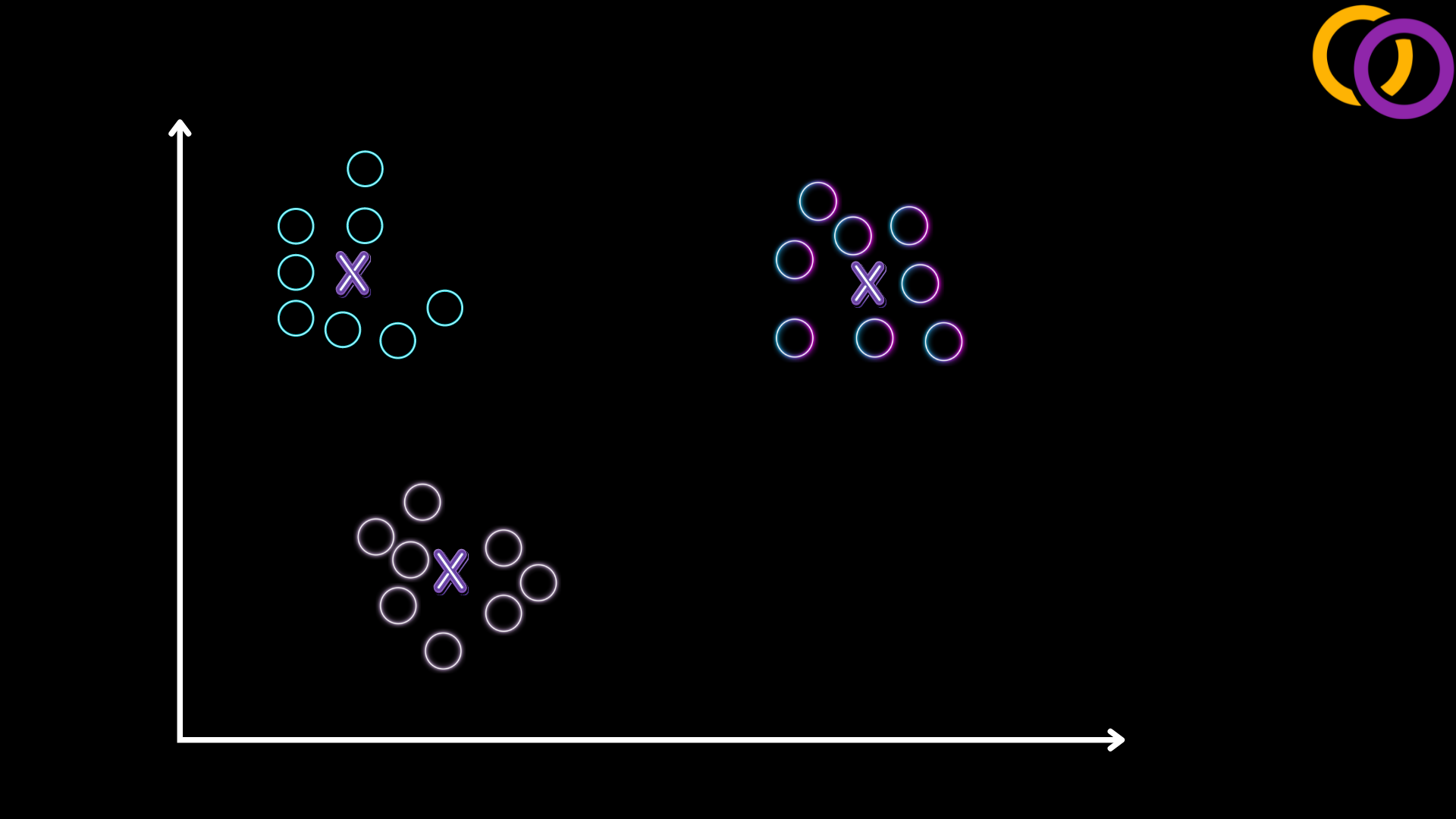
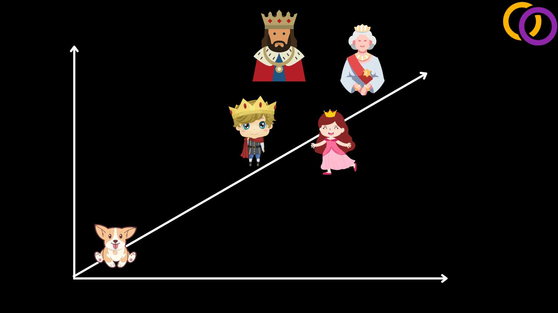
Topic modelling is often performed by clustering algorithms. For example, you may have heard of the k-means algorithm, as shown in Figure 1. In this example, we're dealing with a two-dimensional space; thus, it's quite intuitive for us to locate the centroid to each cluster. But what about language? How can we represent text in a mathematical way such that we can cluster similar text together? Maarten Grootendorst explored these topics in his paper "BERTopic: Neural topic modeling with a class-based TF-IDF procedure" which was the basis for the Python package he created called BertTopic and is what we'll cover in this tutorial.

Methodology

We'll discuss how BERTopic works from a high level. Although knowing these concepts is not strictly necessary to use the library, I believe this background information will give you some appreciation for the package. It will also provide you with some intuition to better understand its capabilities and limitations.

Document Embeddings

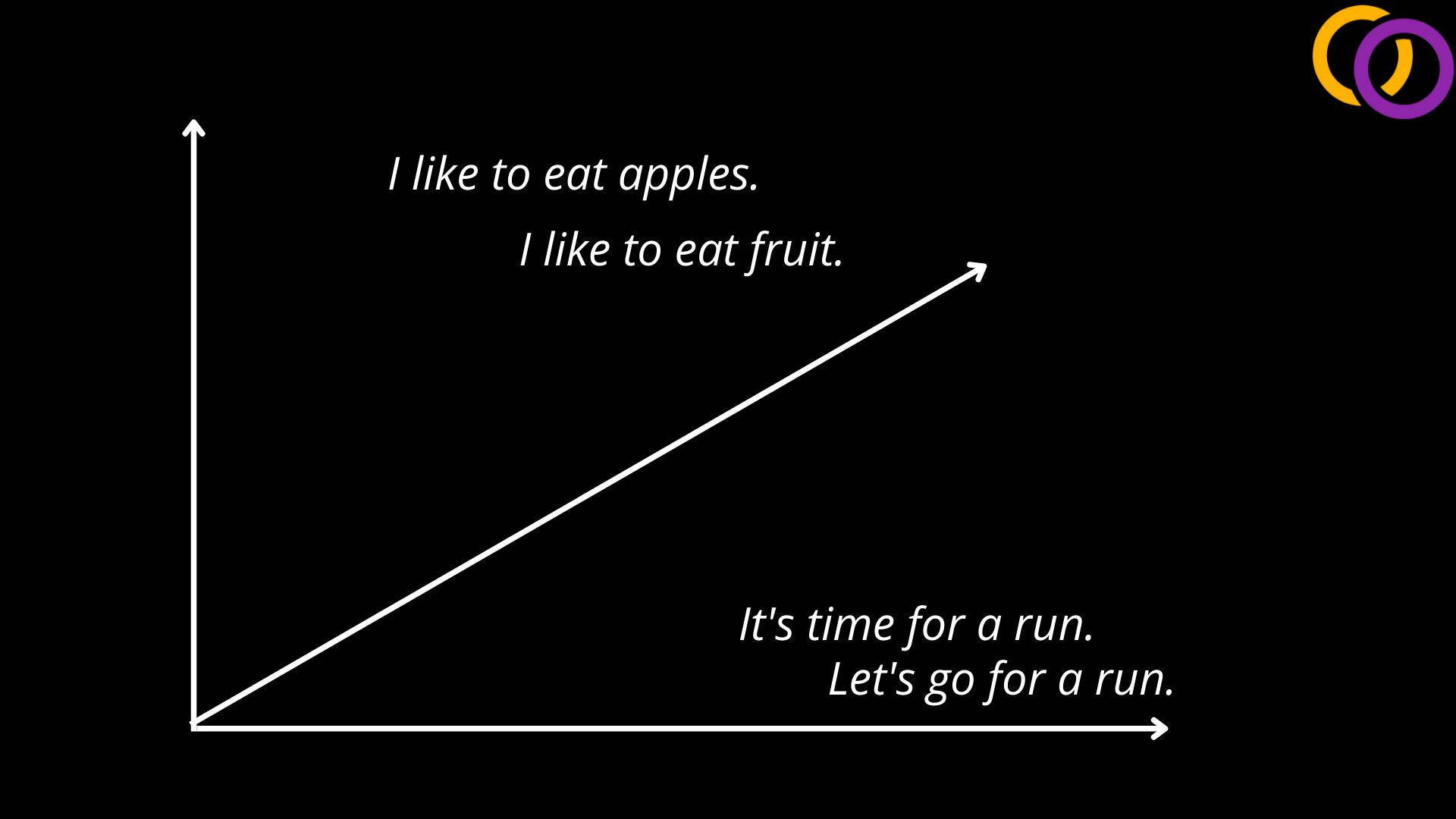
The author used a model called Sentence BERT to generate vectors to represent the meaning of the sentences. This model can be used through a package called Sentence Transformers which I've already published an article on. But to explain it quickly, it is possible using technologies like Word2vec to represent individual entities as vectors where entities with similar meanings are close together within the high dimensional vector space, as shown in Figure 2. Then, the authors of Sentence Transformers found a way to expand upon this concept and efficiently compute vector representations for entire sentences using Transformer models, as shown in Figure 3. These vectors can then be clustered like any other vector for other machine learning topics.

Clustering

The outputted vectors have hundreds of dimensions, making them hard to cluster effectively. So, the author of BERTopic reduced the number of dimensions using a technique called UMAP. Then, the author clustered the vectors using an algorithm called HDBSCAN. One key advantage of using HDBSCAN over k-means is that outlier documents are not assigned to any cluster.

Topic Representations

The author was able to model the meaning of each cluster by using a modified version of the famous algorithm TF-IDF ( term frequency-inverse document frequency). By using this algorithm, the author was able to find keywords to that represent the unique meaning of each cluster.

Here's a great article by the author of BERTopic that explains the methodology in more detail.

Code

Install

First off, we need to pip install the BERTopic library and Hugging Face's Datasets library.

pip install bertopic

pip install datasets

Import

We'll import a class called BERTopic to load the model and a function called load_dataset to load the data we'll use.

from bertopic import BERTopic

from datasets import load_dataset

Data

We'll use a dataset called newspop, which contains titles and headlines for news articles. The articles are about one of four topics: "economy," "microsoft," "obama," or "palestine."

dataset = dataset = load_dataset("newspop", split="train[:]")
print(dataset)

Output:

Dataset({ features: ['id', 'title', 'headline', 'source', 'topic', 'publish_date', 'facebook', 'google_plus', 'linked_in'], num_rows: 93239 })

Let's create list of strings which we'll call docs that will contain all of the headlines for the "economy" topic. We'll ignore the other topics for this tutorial to keep the subject matter more specific.

docs = []
for case in dataset:
  if case["topic"] == "economy":
    docs.append(case["headline"])

Model

By default, BERTopic uses a Transformer model called all-MiniLM-L6-v2 to produce embeddings (which we call vectors). Other models from this webpage may be used instead, like all-mpnet-base-v2. To load a model, simply pass the name of the model in the form of a string to the BERTopic class, or don't pass anything to use the default model.

topic_model = BERTopic()
topic_model_large = BERTopic("all-mpnet-base-v2")

Fit

We can fit the model from here by calling our BERTopic object's fit_transformer() method. This would perform all of the steps we've mentioned in the Methodology section. This method outputs two lists which we wrote to the variables: topics and probs. The topics list contains an integer for each document we provided to indicate which topic it belongs to. Similarly, the probs list contains the probability that the document belongs to the given topic, or in other words, the model's certainty.

topics, probs = topic_model.fit_transform(docs)

Output:

topics: [48, -1, 197, 51, 28, -1, 28, 113

probs: [0.39530761 0. 0.87681452 ... ...

Topic Information

We can get information describing each topic by calling our BERTopic object's get_topic_info() method.

topic_information = topic_model.get_topic_info()

print(type(topic_information))
print(topic_information)

Output:

<class 'pandas.core.frame.DataFrame'>

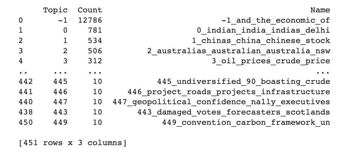
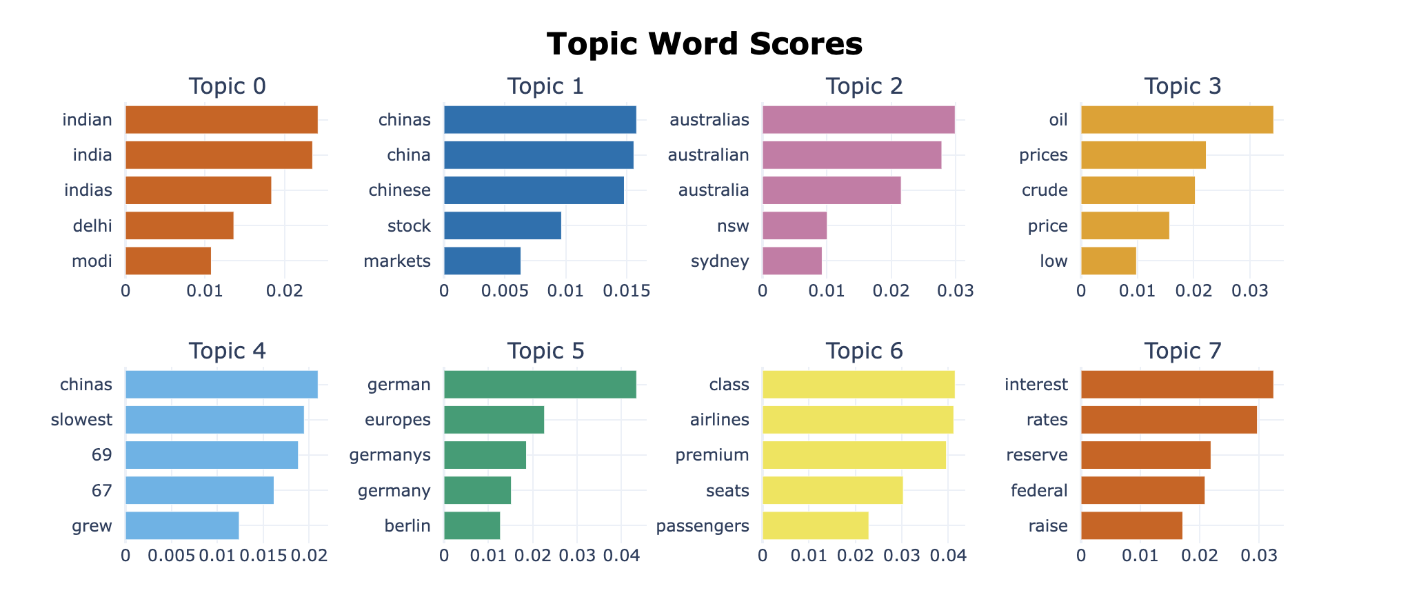
The output is a Pandas Dataframe with the number of documents that fall within each topic. It shows 571 topics in order of how many documents belong to them. The first topic, "-1" is a special topic for outliner topics. From there, we see that the topic with the ID "0" and the keywords indian, india, indias and delhi. An uncased model was used, which is why the keyword "india" was included and not "India."

Topic Words

We can get more information about each topic by calling our BERTopic's get_topic() method. This outputs a list of words for the topic in order of their c-TF-IDF score, or in simple terms, in order of how frequent and unique they are to the document.

topic_words = topic_model.get_topic(1)

print(topic_words)

Output:

[('chinas', 0.015813306322630498), ('china', 0.015591368223916793), ('chinese', 0.014804180963690598), ('stock', 0.009647643864245648), ('markets', 0.006318743167715607), ('investors', 0.005463262912711349), ('beijing', 0.004961607152326786), ('slowing', 0.0049524367246551), ('slowdown', 0.004842723621405817), ('transition', 0.004610423563249632)]

Visualize

We can visualize the topics by calling the visualize_topics() method. This allows us to see how closely related the topics are to each other. But keep in mind that this is a 2D visualization, so it's not a perfect representation of the relationships between the topics.

topic_model.visualize_topics()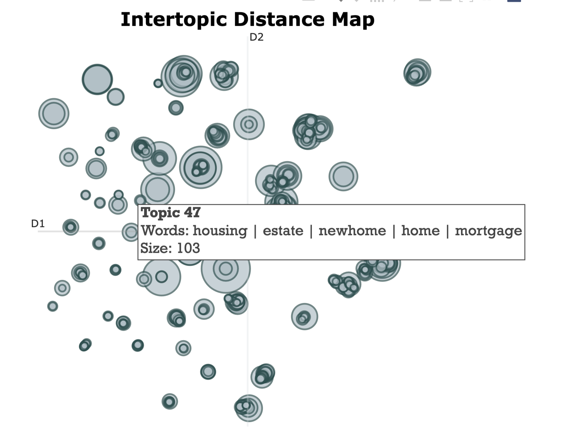

We can also create a bar chart by calling the visualize_barchart() method.

topic_model.visualize_barchart()

Predict:

We can predict what topic any arbitrary text belongs to using the fitted model. We can accomplish this by calling the transform() method. The code below demonstrates this and uses a made up headline for a news article

text = "Canadian exports are increasing thanks to the price of the loonie."
preds, probs = topic_model.transform(text)
print(preds)

Output:

[134]

So, the text belong to topic 134.

top_topic = preds[0]
print(topic_model.get_topic(top_topic))

Output:

[('canadian', 0.04501383345022021), ('loonie', 0.027398899359877694), ('oil', 0.019824369172360856), ('canadas', 0.01929452512991699), ('dollar', 0.01618096137734324), ('canada', 0.015786429651750266), ('low', 0.013508135891745342), ('prices', 0.012762238106106171), ('shock', 0.012483071191448812), ('depreciation', 0.012362746742117799)]

We see that the keywords for the topic the text was classified into appear to match the text well.

Conclusion

We just learned how to use BERTopic to perform topic modelling. Now, I recommend you check out my previous article that covers computing semantic similarity with a Python library called Sentence Transformers. This is the same library that BERTopic uses to compute the document embeddings. On a final note, we plan on posting a video on YouTube about BERTopic in the future so be sure to subscribe to us on YouTube.

Here's the code from this tutorial in Google Colab.

Book a Call

We may be able to help you or your company with your next NLP project. Feel free to book a free 15 minute call with us.